Neural Netwrks are black-boxes and are really cryptic about the features they use to classify the input. Class Activation Maps or more commonly known as Heatmaps can help us understand what the network pay attention to when classifying an image.

Class Activation Maps

Heatmaps are commonly used in UX research to create designs that maximise user attention and interaction. We'll be doing something similar, we'll overlay a class activation map on the original input to see the areas responsible for the output generated.

The pixels responsible for the prediction of a class by the neural-net will be represented with warmer colors and the ones that the ignored by the network will have more cooler colours.

The Model

I'm a simple and I like easy work so we'll be using ResNet-50 with Keras .

ResNet-50 is a Convolutional Neural Network (CNN) that is trained on the ImageNet dateset.

The network is 50 layers deep with over 25 million parameters. Keras provides us with the model in its API and can be used using tensorflow.keras.applications.resnet50.ResNet50().

Making Inferences

Following along on your machine requires installation of a few packages,I recommend you to install all the required packages in a python virtual environment. Don't pollute your global python installation, I've been there and it ain't pretty.

We'll be needing Numpy (pip install numpy), Tensorflow (pip install tensorflow) (Keras is packaged with Tensorflow) and Matplotlib (pip install matplotlib).

You can find all the code used here: Github Gist . To follow along just open the code in Google Colaboratory using the option provided at the top

Loading Images

With that done you'll need an image (or images). I'll be using :

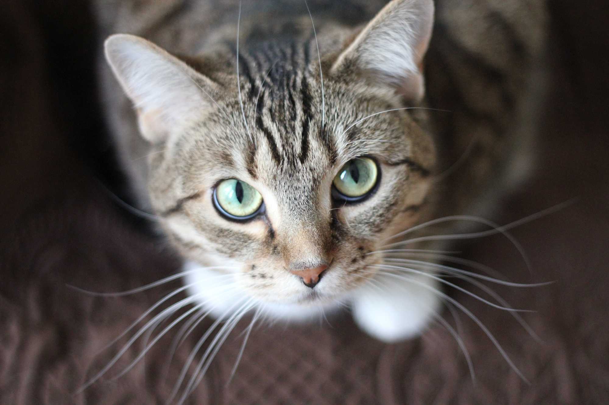
I'll be using the Keras image() function load in the image and later convert it into an array.

Now finally let's look at some code:

Copy
1# getting the packages
2import tensorflow as tf
3from tensorflow.keras.applications.resnet50 import preprocess_input, decode_predictions
4from tensorflow.keras.preprocessing import image
5import numpy as np
6import matplotlib.pyplot as plt
7
8# loading in the image
9IMAGE = "./cat.jpg"  # replace with your image path
10
11# ResNet50 wants the image dimension as (244 x 244) pixels
12img = image.load_img(IMAGE, target_size=(224, 224))
13
14plt.imshow(img)
15plt.show()

And if everything is fine you should see the resized image

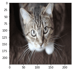
Preprocessing & Inference

With the image loaded let's get the inference running.

But before that we need do a little more work. The model requires a batch of images or more simply an array of images hence, we need to make our input data dimensionally correct

At the moment our is a 3-D array with dimensions $224 * 224 *3$ ($(244 * 244)$ is the pixels and $3$ being the RGB channels). For a batch of images the dimensions would be $size \: of \: the \: batch * 224 * 224 * 3$. To do so we use the Numpy function expand_dims()

Copy
1img_array = image.img_to_array(img)
2img_batch = np.expand_dims(img_array, axis=0)

Now that our data is dimensionally correct we can move to normalising our pixel values. preprocess_input() will do the necesarry work for us.

With that done we can get the model and run an inference.

Copy
1# ...
2#normalise the input image batch
3img_normalised = preprocess_input(img_batch)
4
5# get the model
6model = tf.keras.applications.resnet50.ResNet50()
7
8#running an inference
9prediction = model.predict(img_normalised)
10print(decode_predictions(prediction, top=5)[0])

The prediction produced is as follows:

Copy
1[
2  ('n02123045', 'tabby', 0.5697842), 
3  ('n02124075', 'Egyptian_cat', 0.29003567), 
4  ('n02123159', 'tiger_cat', 0.11475985), 
5  ('n02127052', 'lynx', 0.016232058), 
6  ('n03443371', 'goblet', 0.0012818157)
7]

The ImageNet Dataset on which ResNet50 was trained is very granular and hence doesn't contain the more general class 'cat'. I can confirm that the cat is indeed a tabby cat.

With just 20 lines of code we created a functional image classifier, pretty neat !! The inference code can be consolidated in to function as follows:

Copy
1def classify(IMAGE_PATH):
2  img = image.load_img(IMAGE_PATH, target_size=(224, 224))
3  model = tf.keras.applications.resnet50.ResNet50()
4  img_array = image.img_to_array(img)
5  img_batch = np.expand_dims(img_array, axis=0)
6  img_preprocessed = preprocess_input(img_batch)
7  prediction = model.predict(img_preprocessed)
8  print(decode_predictions(prediction, top=5)[0])

Creating the Class Activation Map

In this section we'll be creating a heatmap for the last convolutional layer of the ResNet50 model and overlay it on the input image.

Creating the Heatmap

So first of all we'll need a model that maps from the input layer ie our image to the activations of the last convolutional layer(as we'll need access to the output values) and the output layer of the model. The names for the layers can be found using model.summary()

Copy
1last_conv_layer_name = "conv5_block3_out"
2classifier_layer_names = [ "avg_pool", "predictions"]
3
4# getting the layer
5last_conv_layer = model.get_layer(last_conv_layer_name)
6# creating the model mapping from inputs to the last convolutional layer's activations
7last_conv_model = tf.keras.Model(model.inputs, last_conv_layer.output)
8
9# Now we would create mapping from the last convolutional layer 
10# (or the classfier's input) to output classes
11classifier_input = tf.keras.Input(shape=last_conv_layer.output.shape[1:])
12x = classifier_input
13
14for layer_name in classifier_layer_names:
15  x = model.get_layer(layer_name)(x)
16
17classifier_model = tf.keras.Model(classifier_input, x)

Now that we have have the necesarry model mapping it's time to calculate the gradient values of the top predicted class with respect to the activations of the last convolutional layer. The gradient values are an accurate depiction of the important features that classifier uses to classify the image.

I'll be using GradientTape() API for automatic differentiation.

Copy
1with tf.GradientTape() as tape:
2  # pass in the normalised image
3  last_conv_layer_output = last_conv_model(img_normalised)
4  tape.watch(last_conv_layer_output)
5
6  # predict the class based on the convolution output
7  preds = classifier_model(last_conv_layer_output)
8  # get the index and class for the top prediction
9  top_pred_index = tf.argmax(preds[0])
10  top_class_channel = preds[:, top_pred_index]
11
12# Computing the gradient values top predicted class with respect to the last convolutional layer's feature map / activations
13grads = tape.gradient(top_class_channel, last_conv_layer_output)
14# Now we average out the gradient values over a specific feature map channel
15pooled_grads = tensorflow.reduce_mean(grads, axis=(0, 1, 2))

With the gradient values we are ready to calculate the the heatmap. To do so we multiply each channel of the feature map / activations by how important that channel is for the class that is predicted for the image. Then the channel-wise mean of the resulting feature-map would be our final class activation map.

Copy
1# get the activation of the last convolutional layer
2last_conv_layer_output = last_conv_layer_output.numpy()[0]
3pooled_grads = pooled_grads.numpy()
4
5# multiplying channels with their gradient values
6for i in range(pooled_grads.shape[-1]):
7  last_conv_layer_output[:, :, i] *= pooled_grads[i]
8
9# channel-wise mean to obtaint the heatmap
10heatmap = np.mean(last_conv_layer_output, axis=-1)

Creating the Output Image

Now that we have the heatmap we can move on to overlaying it on our original image. We need to make a colour map from the heatmap values. I'll be using the jet colour map from matplotlib.

Copy
1import matplotlib.cm as cm
2
3# normalise the heatmap values to the range [0,1]
4heatmap = np.maximum(heatmap, 0) / np.max(heatmap)
5
6jet = cm.get_cmap("jet")
7# Scale the values of the heatmap
8heatmap = np.uint8(255 * heatmap)
9
10# Get the color heatmap
11jet_colours = jet(np.arange(256))[:, :3]
12colour_heatmap = jet_colours[heatmap]

Now that we have the colour heatmap we can get the input image, superimpose the colour heatmap and save the image

Copy
1# getting the orginal image
2img2 = tf.keras.preprocessing.image.load_img(IMAGE)
3img2 = tf.keras.preprocessing.image.img_to_array(img2)
4
5# resizing the heatmap to fit the image 
6colour_heatmap = image.array_to_img(colour_heatmap)
7colour_heatmap = colour_heatmap.resize((img2.shape[1], img2.shape[0]))
8colour_heatmap = image.img_to_array(colour_heatmap)
9
10#superimposing the colour heatmap
11superimposed_img = colour_heatmap * 0.4 + img2
12superimposed_img = image.array_to_img(superimposed_img)
13
14OUTPUT = "cat_heatmap.jpg"
15superimposed_img.save(OUTPUT)

Now to view the final image:

Copy
1import matplotlib.image as mpimg
2
3grad_img = mpimg.imread(OUTPUT)
4plt.imshow(grad_img)
5plt.show()

And voila!!

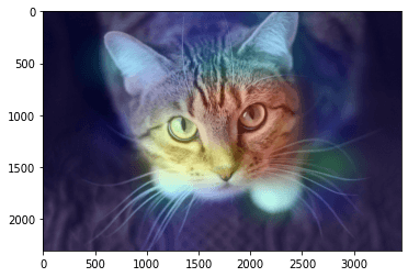
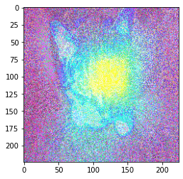
Try changing the values of last_conv_layer_name and classifier_layer_names and see how the features change through the different convolution layers.

The Easier Way

The above implementation can be a little overwhelming, but it is quite straightforward once you get the hang of it. But there is a simpler way to do this with the help of tf_explain (pip install tf_explain) and GradCAM(). But the results were ok at best and the documentation is not that great.

Copy
1from tf_explain.core.grad_cam import GradCAM
2
3data = (img_batch, None)
4explainer = GradCAM()
5# here 281 is the class index of tabby cat
6grid = explainer.explain(data, model, 281)
7explainer.save(grid, ".", "output_gradCAM.png")
8
9gradCAM_img = mpimg.imread("output_gradCAM.png")
10plt.imshow(gradCAM_img)
11plt.show()

The output produced is fine and can be helpful for prototyping.

You can get the complete code here : atishekk/resNet50-class-activation-map.ipynb